
}}</ref>{{efn-ua| ”Note: Although the total spatio-temporal modes increase with Δf·t, detector bandwidth, decoherence, and losses can limit the number of effectively measurable modes.”}}
}}</ref>{{efn-ua| ”Note: Although the total spatio-temporal modes increase with Δf·t, detector bandwidth, decoherence, and losses can limit the number of effectively measurable modes.”}}
== Example calculation (50 µm sphere, near-infrared light) ==
== Example calculation (50 µm sphere, near-infrared light) ==
* ”R” = 50 µm, ”λ” = 800 nm → ”kR” ≈ 393
* ”R” = 50 µm, ”λ” = 800 nm → ”kR” ≈ 393
* ”N” ≈ 2.8 × 10<sup>7</sup>
* ”N” ≈ 2.8 × 10<sup>7</sup>
* Δ”f” = 10 THz, ”t” = 1 s → Δ”f”·”t” = 10<sup>13</sup>
* Δ”f” = 10 THz, ”t” = 1 s → Δ”f”·”t” = 10<sup>13</sup>
* ”N”<sub>total</sub> ≈ 2.8 × 10<sup>20</sup><br>{{efn-ua|”Note: This example gives a theoretical estimate (practical detection may yield far fewer modes than the theoretical ”N”<sub>total</sub> ).”}}
* ”N”<sub>total</sub> ≈ 2.8 × 10<sup>20</sup><br>{{efn-ua|”Note: This example gives a theoretical estimate (practical detection may yield far fewer modes than the theoretical ”N”<sub>total</sub> ).”}}
Maximum number of independent classical or quantum spatial modes inside a spherical volume

Beams inside a sphere is based on Quantum optics a branch of atomic, molecular, and optical physics and quantum chemistry that studies the behavior of photons (individual quanta of light). and refers to the number of simultaneously supportable propagable orthogonal spatial modes in the wavefield confined in a spherical region of radius R with negligible crosstalk. The concept applies equally well in both the classical and quantum channels and deals with electromagnetic waves (light or radio waves), acoustic waves (sound or ultrasonic waves), or de Broglie matter waves.
Every beam corresponds to a different orthogonal mode in the spatial structure of the electromagnetic field (for example, Laguerre–Gaussian modes, Hermite–Gaussian modes, or spherical-harmonic modes). The number of such modes in principle depends upon the size of the accessible phase space defined in the sphere and finally upon the diffraction limit contained in the wavelength λ.
This applies in many fields. For quantum optics and quantum information research, this determines the maximum dimensionality of quantum entanglement in the spatial mode and the quantum ca|pacity of free-space quantum communication channels. For classical free-space optical communication links, the same counting gives the ultimate (hole-burning-free) upper bound on the number of independent spatial channels, the diffraction-limited number of spatial degrees of freedom (a three-dimensional analogue of the familiar A/λ² limit for planar apertures).
For phased arrays in radar or radio astronomy applications, this defines the number of independently beam-steerable or spatially resolvable beams or channels. For medical ultrasonic imaging or sonar applications, this closely-related idea defines the number of independently addressable focal areas or image pixels. Theoretically, in the latest volumetric or five-dimensional optical information recording technologies, this determines the overall data packing density if all possible spatial and polarization freedoms are utilized.
Since the same counting in the phase-space argument holds equally for classical waves and quantum states consisting of one or few photons, this limit turns out to be universal.[1][2][3][A]
The fundamental limit imposed by a finite volume on the number of independent communication channels was first analysed in optics during the 1960s and 1970s.[4][5] These works showed that the number of spatial degrees of freedom of a field confined to a region of radius R scales as (2πR/λ)² in two dimensions and (2πR/λ)³ in three dimensions.
In 2000, David A. B. Miller derived a precise expression for the number of orthogonal spatial channels that can be supported between two spherical volumes in free space, obtaining N ≈ (kR)³ / (3π²) when both polarisations are included.[2] This result has become the standard reference for the maximum number of “beams in a sphere”.
Since the mid-2010s, the same spatial-mode counting argument has been widely applied in high-dimensional quantum optics, where approximately (kR)³ modes (orbital-angular-momentum, Laguerre–Gaussian, or pixel bases) are used as independent quantum channels.[1][3]
When finite bandwidth Δf and observation time t are taken into account, the total number of independent spatio-temporal channels is approximately Nspatial × Δf × t. This formula is now routinely used to estimate fundamental limits in quantum communication, radar, and imaging.[3]
[B]
The fundamental diffraction limit is
- N ≈ 2 × ( k R ) 3 3 π 2 ≈ 0.068 ( 2 π R λ ) 3 {\displaystyle N\approx 2\times {\frac {(kR)^{3}}{3\pi ^{2}}}\approx 0.068\left({\frac {2\pi R}{\lambda }}\right)^{3}}


independent spatial modes (including both polarisation states), where
k
=
2
π
λ
{\displaystyle k={\frac {2\pi }{\lambda }}}
is the wavenumber.[2][3]
With finite bandwidth Δf and observation time t, the total number of independent spatio-temporal channels becomes


- N total ≈ N × Δ f × t {\displaystyle N_{\text{total}}\approx N\times \Delta f\times t} .[3]


Quantum-mechanical limit
[edit]
A quantum limit in physics is a limit on measurement accuracy at quantum scales.[6]

Per polarisation:
- N per pol ≈ ( k R ) 3 3 π 2 {\displaystyle N_{\text{per pol}}\approx {\frac {(kR)^{3}}{3\pi ^{2}}}}


including both polarisations:
- N ≈ 2 × ( k R ) 3 3 π 2 ≈ 0.068 ( 2 π R λ ) 3 {\displaystyle N\approx 2\times {\frac {(kR)^{3}}{3\pi ^{2}}}\approx 0.068\left({\frac {2\pi R}{\lambda }}\right)^{3}} .[2][3][7][1] [C]
Classical beam packing
[edit]
For non-diffracting beams of diameter d, geometric packing gives a crude (and irrelevant) upper bound N ≲ ( 2 R / d ) 3 {\displaystyle N\lesssim (2R/d)^{3}} .[8][D]


Including time and bandwidth
[edit]


- R = 50 µm, λ = 800 nm → kR ≈ 393
- N ≈ 2.8 × 10⁷
- Δf = 10 THz, t = 1 s → Δf·t = 1013
- Ntotal ≈ 2.8 × 10²⁰
[F]
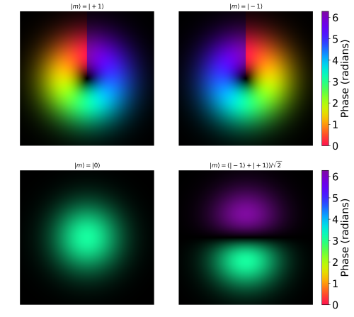
Quantum wavefunctions in spheres
[edit]
Spherical harmonics and Bessel functions are the natural solutions of the Helmholtz or Schrödinger equation (these functions form a complete orthogonal set for the spatial modes in the sphere).
- ^ Note: The calculations and limits below assume an ideal sphere, a homogeneous medium, and neglect losses, decoherence, or other non-ideal effects. An “independent mode” is defined here as an orthogonal spatial mode with minimal crosstalk
- ^ Note: Recent studies show that practical implementations of high-dimensional spatial modes can be limited by non-ideal media, optical aberrations, and detector limitations.
- ^ Note: Both polarizations are included in the count. The number N represents a theoretical limit; practically achievable values may be lower due to material imperfections or measurement errors.
- ^ Note: This geometric limit is theoretical; in practice, diffraction and interference can reduce the number of effectively usable beams.
- ^ Note: Although the total spatio-temporal modes increase with Δf·t, detector bandwidth, decoherence, and losses can limit the number of effectively measurable modes.
- ^ Note: This example gives a theoretical estimate (practical detection may yield far fewer modes than the theoretical Ntotal ).
- ^ a b c Erhard, Manuel; Krenn, Mario; Zeilinger, Anton (2020). “Advances in high-dimensional quantum entanglement”. Nature Reviews Physics. 2: 365–381. doi:10.1038/s42254-020-0193-5.
- ^ a b c d Miller, David A. B. (2000). “Communicating with waves between volumes: evaluating orthogonal spatial channels and limits on coupling strengths”. Applied Optics. 39 (11): 1681–1699. Bibcode:2000ApOpt..39.1681M. doi:10.1364/AO.39.001681.
- ^ a b c d e f Fabre, Claude; Treps, Nicolas (2020). “Modes and states in quantum optics”. Reviews of Modern Physics. 92 (3): 035005. arXiv:1912.09321. doi:10.1103/RevModPhys.92.035005.
{{cite journal}}: CS1 maint: article number as page number (link) - ^ Toraldo di Francia, G. (1969). “Degrees of freedom of an image”. Journal of the Optical Society of America. 59 (7): 799–804. doi:10.1364/JOSA.59.000799.
- ^ Lukosz, W. (1966). “Optical systems with resolving powers exceeding the classical limit”. Journal of the Optical Society of America. 56 (11): 1463–1472. doi:10.1364/JOSA.56.001463.
- ^ Braginsky, V. B.; Khalili, F. Ya. (1992). Quantum Measurement. Cambridge University Press. ISBN 978-0-521-48413-8.
- ^ Erhard, Manuel; Fickler, Robert; Krenn, Mario; Zeilinger, Anton (2017). “Twisted photons: new quantum perspectives in high dimensions”. Light: Science & Applications. 6 (10): e17146. doi:10.1038/lsa.2017.146. PMC 5655069. PMID 29138663.
- ^ Conway, John H.; Sloane, Neil J. A. (1999). Sphere Packings, Lattices and Groups (3rd ed.). Springer. ISBN 978-0-387-98585-5.
- ^ Brecht, Bernd; Reddy, Divya V.; Silberhorn, Christoph; Raymer, Michael G. (2015). “Photon temporal modes: a complete framework for quantum information science”. Physical Review X. 5: 041017. doi:10.1103/PhysRevX.5.041017.
{{cite journal}}: CS1 maint: article number as page number (link)